The Best Trajectory to Negotiate a Turn in the Road

Introduction

            This animation will show the resulting lateral accelerations for two types of curve.  First is the ideal curve that is the largest one that can stay within the bounds of the lane.  Second is a curve that is adjustable by the user.  For both types of curve, the speed profile is adjustable via a smooth Bezier curve.

Figures
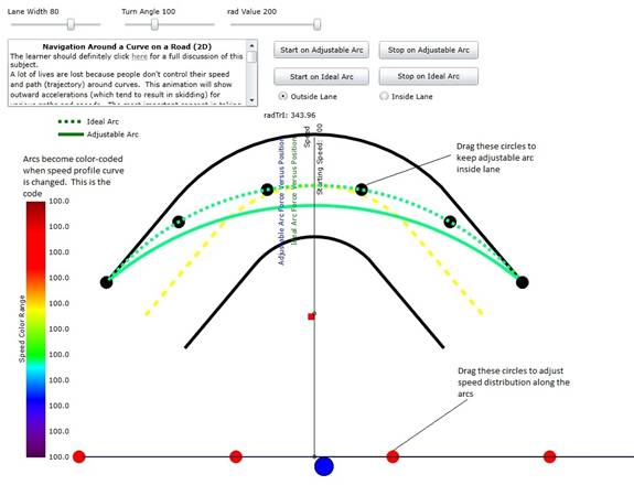
Figure 1: Diagram of the animation describing how to use the adjustable arc and speed profile.

Computing the ideal arc
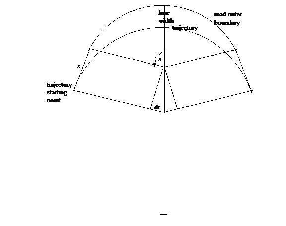
Figure 1: Diagram of the turn outer boundary and the possible trajectory.  Symbol a is half of the total turn angle while symbol s is the straight line distance from the start of the curved trajectory to the start of the arc that represents the outer boundary of the road.  as can be seen, the parameter dr is the difference between the trajectory radius and the road outer bound radius.

It is obvious from the figure that the value of dr is:

dr= s tana MathType@MTEF@5@5@+= feaagKart1ev2aaatCvAUfeBSjuyZL2yd9gzLbvyNv2CaerbuLwBLn hiov2DGi1BTfMBaeXatLxBI9gBaerbd9wDYLwzYbItLDharqqtubsr 4rNCHbGeaGqiVCI8FfYJH8YrFfeuY=Hhbbf9v8qqaqFr0xc9pk0xbb a9q8WqFfeaY=biLkVcLq=JHqpepeea0=as0Fb9pgeaYRXxe9vr0=vr 0=vqpWqaaeaabiGaciaacaqabeaadaqaaqaaaOqaaiaadsgacaWGYb Gaeyypa0ZaaSaaaeaacaWGZbaabaGaciiDaiaacggacaGGUbGaamyy aaaaaaa@3D90@  

(1.5)

Also the lane width, w, is

w= s sina s tana MathType@MTEF@5@5@+= feaagKart1ev2aaatCvAUfeBSjuyZL2yd9gzLbvyNv2CaerbuLwBLn hiov2DGi1BTfMBaeXatLxBI9gBaerbd9wDYLwzYbItLDharqqtubsr 4rNCHbGeaGqiVCI8FfYJH8YrFfeuY=Hhbbf9v8qqaqFr0xc9pk0xbb a9q8WqFfeaY=biLkVcLq=JHqpepeea0=as0Fb9pgeaYRXxe9vr0=vr 0=vqpWqaaeaabiGaciaacaqabeaadaqaaqaaaOqaaiaadEhacqGH9a qpdaWcaaqaaiaadohaaeaaciGGZbGaaiyAaiaac6gacaWGHbaaaiab gkHiTmaalaaabaGaam4CaaqaaiGacshacaGGHbGaaiOBaiaadggaaa aaaa@425F@  

(1.6)

From equation  (1.6) we may compute s in terms of w and a:

s=w sina 1cosa MathType@MTEF@5@5@+= feaagKart1ev2aaatCvAUfeBSjuyZL2yd9gzLbvyNv2CaerbuLwBLn hiov2DGi1BTfMBaeXatLxBI9gBaerbd9wDYLwzYbItLDharqqtubsr 4rNCHbGeaGqiVCI8FfYJH8YrFfeuY=Hhbbf9v8qqaqFr0xc9pk0xbb a9q8WqFfeaY=biLkVcLq=JHqpepeea0=as0Fb9pgeaYRXxe9vr0=vr 0=vqpWqaaeaabiGaciaacaqabeaadaqaaqaaaOqaaiaadohacqGH9a qpcaWG3bWaaSaaaeaaciGGZbGaaiyAaiaac6gacaWGHbaabaGaaGym aiabgkHiTiGacogacaGGVbGaai4Caiaadggaaaaaaa@4214@  

(1.7)

and from equations 1.5 and 1.7 we can compute dr:

dr=w sina tana(1cosa) =w cosa 1cosa MathType@MTEF@5@5@+= feaagKart1ev2aaatCvAUfeBSjuyZL2yd9gzLbvyNv2CaerbuLwBLn hiov2DGi1BTfMBaeXatLxBI9gBaerbd9wDYLwzYbItLDharqqtubsr 4rNCHbGeaGqiVCI8FfYJH8YrFfeuY=Hhbbf9v8qqaqFr0xc9pk0xbb a9q8WqFfeaY=biLkVcLq=JHqpepeea0=as0Fb9pgeaYRXxe9vr0=vr 0=vqpWqaaeaabiGaciaacaqabeaadaqaaqaaaOqaaiaadsgacaWGYb Gaeyypa0Jaam4DamaalaaabaGaci4CaiaacMgacaGGUbGaamyyaaqa aiGacshacaGGHbGaaiOBaiaadggacaGGOaGaaGymaiabgkHiTiGaco gacaGGVbGaai4CaiaadggacaGGPaaaaiabg2da9iaadEhadaWcaaqa aiGacogacaGGVbGaai4CaiaadggaaeaacaaIXaGaeyOeI0Iaci4yai aac+gacaGGZbGaamyyaaaaaaa@5338@  

(1.8)


Computing the Lateral Acceleration

I assume we have a parametric path in 2D space:


x i , y i MathType@MTEF@5@5@+= feaagKart1ev2aaatCvAUfeBSjuyZL2yd9gzLbvyNv2CaerbuLwBLn hiov2DGi1BTfMBaeXatLxBI9gBaerbd9wDYLwzYbItLDharqqtubsr 4rNCHbGeaGqiVCI8FfYJH8YrFfeuY=Hhbbf9v8qqaqFr0xc9pk0xbb a9q8WqFfeaY=biLkVcLq=JHqpepeea0=as0Fb9pgeaYRXxe9vr0=vr 0=vqpWqaaeaabiGaciaacaqabeaadaqaaqaaaOqaaiaadIhadaWgaa WcbaGaamyAaaqabaGccaGGSaGaamyEamaaBaaaleaacaWGPbaabeaa aaa@3AD4@  

(1.1)

where i is the counter integer for successive points, what  is the transverse acceleration needed to stay on the path?

The transverse acceleration depends on the rate of change of the vector normal to the path.  If we just have a listing of x i , y i MathType@MTEF@5@5@+= feaagKart1ev2aqatCvAUfeBSjuyZL2yd9gzLbvyNv2CaerbuLwBLn hiov2DGi1BTfMBaeXatLxBI9gBaerbd9wDYLwzYbItLDharqqtubsr 4rNCHbGeaGqiVCI8FfYJH8YrFfeuY=Hhbbf9v8qqaqFr0xc9pk0xbb a9q8WqFfeaY=biLkVcLq=JHqpepeea0=as0Fb9pgeaYRXxe9vr0=vr 0=vqpWqaaeaabiGaciaacaqabeaadaqaaqaaaOqaaiaadIhadaWgaa WcbaGaamyAaaqabaGccaGGSaGaamyEamaaBaaaleaacaWGPbaabeaa aaa@3AD5@  then we can make an estimate of the change of the unit normal, n, by taking the following quantities:

First the local normal is computed from:

dx=x x 0 ,dy=y y 0 ds= d x 2 +d y 2 n= dy ds x+ dx ds y MathType@MTEF@5@5@+= feaagKart1ev2aaatCvAUfeBSjuyZL2yd9gzLbvyNv2CaerbuLwBLn hiov2DGi1BTfMBaeXatLxBI9gBaerbd9wDYLwzYbItLDharqqtubsr 4rNCHbGeaGqiVCI8FfYJH8YrFfeuY=Hhbbf9v8qqaqFr0xc9pk0xbb a9q8WqFfeaY=biLkVcLq=JHqpepeea0=as0Fb9pgeaYRXxe9vr0=vr 0=vqpWqaaeaabiGaciaacaqabeaadaqaaqaaaOabaeqabaGaamizai aadIhacqGH9aqpcaWG4bGaeyOeI0IaamiEamaaBaaaleaacaaIWaaa beaakiaacYcacaaMc8UaaGPaVlaadsgacaWG5bGaeyypa0JaamyEai abgkHiTiaadMhadaWgaaWcbaGaaGimaaqabaaakeaacaWGKbGaam4C aiabg2da9maakaaabaGaamizaiaadIhadaahaaWcbeqaaiaaikdaaa GccqGHRaWkcaWGKbGaamyEamaaCaaaleqabaGaaGOmaaaaaeqaaaGc baGaaCOBaiabg2da9iabgkHiTmaalaaabaGaamizaiaadMhaaeaaca WGKbGaam4CaaaacaWH4bGaey4kaSYaaSaaaeaacaWGKbGaamiEaaqa aiaadsgacaWGZbaaaiaahMhaaaaa@5E4C@  

(1.2)

where x0 and y0 are immediately previous values of x,y and x and y are the present values.  In order to compute the change in normal vector we need to have saved an immediately previous value of n as n0

Then

dn=n- n 0 MathType@MTEF@5@5@+= feaagKart1ev2aaatCvAUfeBSjuyZL2yd9gzLbvyNv2CaerbuLwBLn hiov2DGi1BTfMBaeXatLxBI9gBaerbd9wDYLwzYbItLDharqqtubsr 4rNCHbGeaGqiVCI8FfYJH8YrFfeuY=Hhbbf9v8qqaqFr0xc9pk0xbb a9q8WqFfeaY=biLkVcLq=JHqpepeea0=as0Fb9pgeaYRXxe9vr0=vr 0=vqpWqaaeaabiGaciaacaqabeaadaqaaqaaaOqaaiaahsgacaWHUb GaaCypaiaah6gacaWHTaGaaCOBamaaBaaaleaacaWHWaaabeaaaaa@3C1E@  

(1.3)

is the local change.  The acceleration a normal to the path then is


a= ( ds dt ) 2 dn ds MathType@MTEF@5@5@+= feaagKart1ev2aaatCvAUfeBSjuyZL2yd9gzLbvyNv2CaerbuLwBLn hiov2DGi1BTfMBaeXatLxBI9gBaerbd9wDYLwzYbItLDharqqtubsr 4rNCHbGeaGqiVCI8FfYJH8YrFfeuY=Hhbbf9v8qqaqFr0xc9pk0xbb a9q8WqFfeaY=biLkVcLq=JHqpepeea0=as0Fb9pgeaYRXxe9vr0=vr 0=vqpWqaaeaabiGaciaacaqabeaadaqaaqaaaOqaaiaahggacqGH9a qpdaqadaqaamaalaaabaGaamizaiaadohaaeaacaWGKbGaamiDaaaa aiaawIcacaGLPaaadaahaaWcbeqaaiaaikdaaaGcdaWcaaqaaiaahs gacaWHUbaabaGaamizaiaadohaaaaaaa@41FF@  

(1.4)

where ds is the spacing along the path of the points and dt is the time increment between points.   Please take note that it is not assumed that the curve is part of a circle.