Diffusion of Two Gases
Introduction
This will
analyze the diffusion of two samples of
gases where one gas is initially on the left side of the container and
the other is on the right side of the container.
Analysis:
Case 1: Simplest case of heat flow into slab:
The gas
diffusion problem is fairly complex so, as a warm-up, I will start by

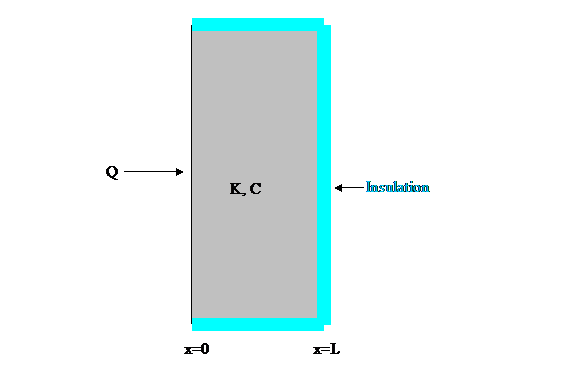
Figure 2: Slab whose
temperature functions are analyzed below.
analyzing the flow of heat into a large, thin slab of
thickness L (see Figure 2).
The solid
state analog of the atoms that we will discuss later are called phonons which
are quantum mechanical entities that represent vibrations of the atomic nuclei
in the solid. These phonon density is higher in the hotter
regions of the solid and they carry the heat from the hotter parts of the
solids to the cooler parts in the same way that one atomic species migrates
from a region where its density is high to a region where its density is
low. The phonons collide with other
phonons which retards their progress in the same way that the atoms of a gas
collide with other atoms retarding their progress toward lower density.
For the
present heat flow problem, the power input into the left side of the slab will
be Q (watts-m-2). The conductivity
will be K (watt m-1 K-1) and the heat capacity will be C
(Joules m-3 K-1).
Further I will assume, as shown, that the slab is insulated on the sides
not in contact with the heat source.
Then we can immediately write that, after transients have died out, the
temperature everywhere in the slab rises
as
(1)
The partial differential equation for heat flow is:
(2)
where the latter equality applies only to steady state. Integrating equation 2 with respect to x once
we obtain:
(3)
where A is a constant that will be determined later by
boundary conditions.
Integrating equation 3 with respect to x results in:
(4)
where B is another constant that we must determine. Note that, since the boundary at x=L is
insulated there is no heat flow there so
(5)
Using equation 5 in equation 3 we get for A:
(6)
Finally we can set B in equation 4 to the initial
temperature, T0, and obtain
(7)
Equation 7
needs a complementary solution to specify the transients that occur when Q is
turned on. For that we use a technique
call "separation of variables" which I will explain next. We have the equation:
(8)
We make the assumption that T can be written:
Then equation 8 can be rewritten:
(9a,b)
where Λ is a constant that will depend on initial
boundary conditions and I have used the symbol D=K/C, which is the diffusivity.
The obvious solution set for equation 9a is
(10a)
and the solution for equation 9b is
(10b)
If we are going to match boundary conditions in the interval
x=(0,L) then the value of Λ has to be
where n is an integer.
Then equations 10a and 10b become:
(10a)
(10b)
Finally we apply the conditions
which implies that
so that
and n is odd. Then
the combined transient solution is
(11)
where we note that
so that T(x,t)=0
at x=L.
Case 2: Diffusion of Gases

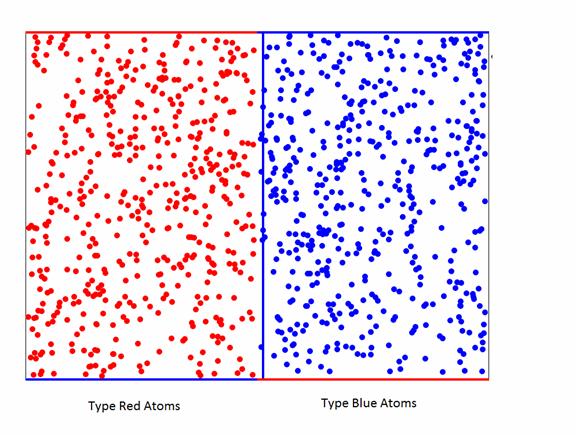
Figure 2. Showing the initial conditions. For this picture there are 500 randomly
placed Red atoms on the left and 500 randomly placed blue atoms on the
right. They have random velocities in
the plane of the Figure.
The equation for the density, n, of atoms is exactly similar
to that for temperature discussed above:
(12)
I will not derive the required solution for n(x,t). It is
(13)
where
where D is the diffusivity and n0 is the starting
density atoms on each side of the mid-line of the container. The function erfc is defined as
I will now differentiate both sides of equation 12 to
confirm that equation 13 is indeed a solution of equation 12.
The
diffusivity, D, here deserves to be better explained. It depends on the average speed <vx>
of the atoms in the horizontal direction as well as the mean free path, lmfp,
between collisions. The latter depends
here on the 2 dimensional density of atoms, n2, which equals
where N is the total number of atoms, h is the height of the
container, and w is its width. The
equation to determine lmfp also depends on the 2 dimensional analog
of the collision cross section, σ2. For 2 dimensions:
where rR is the radius of the red atoms and rB
is the radius of the blue atom.
Then the equation for
the mean free path is:
The equation to obtain D from these quantities is:
Effect of Different Atomic Mass
So far we
have been assuming that the masses of the red and blue atoms are the same so
that, upon collision, speed changes of both types of atoms are the same. Suppose now that the masses, M, of the atoms
(since we are just working in two dimensions and therefore the atoms are really
discs of the same thickness) is proportional to their radii squared:
Similarly we expect the average speeds, since the atomic speeds
are generated by temperature, to be in the ratio:
Note that the product of mass times speed is the
momentum, p, and the ratio of the average momentums is
If, for example, rR>rB this
asymmetry results in a net random walk of momentum
(Mv) from left to right. Therefore the equation developed in the
previous section will not be valid.

