Fit of Binomial Distribution (Pascal’s Triangle) to a Gaussian
Introduction
Many processes in the real world can rely on situations where there are only two possible outcomes. A really important example of this is heredity of biological genes but quite a few genetic inheritance cases are more complex than simple binary. So, here, we will consider the simple situation where N coins are tossed and can land with either heads or tails showing.
It is
useful and instructive to develop a simple algebraic model of the probabilities
of the number of heads. Although it is
well known that the probabilities are given by the binomial distribution, this
distribution becomes unwieldy when the number of coins tossed per throw is
large because of the very large factorials involved. Therefore I chose to fit these probabilities
to a simple Gaussian curve since that is the basis of many statistical
analyses. The factorials in the binomial
distribution can be well approximated using
Use of Stirling ’s Approximate Formula for the Factorial
![]() (1)
(1)
and is accurate to within about 1/2%
when k is 7 and much more accurate for larger k. A very simple
http://en.wikipedia.org/wiki/Stirling's_approximation
Maximum Value of Probability
Since our experiment involves the probability of only 2 different ways the objects can land, if N is the number of items thrown, then the total number of possible ways that the items can land is 2N. Using the binomial theorem we have the maximum probability:
 (2)
(2)
where, in the denominator, the N/2
and (N+1)/2 are integer values.
Using expression 1 in equation 2 we have:
 (3)
(3)
where
 (4)
(4)
For notation simplicity we will henceforth use the symbol Nc=ceil(N/2).
Width of Gaussian
The width
of the Gaussian involves taking the logarithms of the
![]() (5)
(5)
where I have set this ratio to 1/e.
Inverting equation 5 and using
![]() (6)
(6)
Taking the logarithm of both sides of equation 6 we get:
![]() (7)
(7)
For fairly large Nc it is valid to make the approximation:

Then equation 7 becomes:
 (8)
(8)
Collecting terms in equation 8 we have:
![]() (9)
(9)
so that
![]() (10)
(10)
Note that in equation 6 we have neglected the square root
terms in equation 1. If included, these
will lead to an additional term -dN2/(2Nc2) on the left side of equation
9. Since Nc>>1 this term will not appreciably
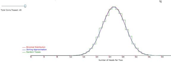
change the result in equation 10. See Figure 1 below for the results.

Figure 1: Fit of binomial distribution to a Gaussian
with parameters computed from the