LCR Oscillator Animation

Introduction

The LCR oscillator (LCR) is an exact analog of the harmonic oscillator shown under the Mechanics chapter. Its behavior goes a long way toward understanding the electrodynamics of the real world.

Current Meter

Inductor L

Resistor R

Capacitor C

Switch

B field lines

Battery

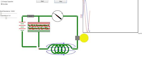
Figure 1: Circuit diagram showing the charging battery, C, R, and L. Also shown is the charging switch and the direction of the current that fills or depletes C. R is a light bulb which changes brightness as current flows through it.

Color Coding

It is well to discuss the color coding of the animation. I have chosen green for negative charge (electrons) and red for positive charge. In metals like the metal plates of the capacitor, which normally have equal negative (electron) and positive (proton) charge numbers, positive charge means some of the normal electron density has been removed.

Also, in the metal wires connecting the LCR elements, only the electrons are mobile so these are shown as small green balls that move at the appropriate current speed when either oscillating or charging the capacitor.

The capacitor plates gradually change from gray to red or green as electrons are removed or added, respectively.

The dipoles (red and green dumb bells) in the capacitor slab have a positive charge at one end and a negative charge at the other and these rotate depending on the charge on the capacitor plates.

Calculations:

The picture above shows the important parameters of the LCR. They include a capacitor, C, a drag element (shown here as

Spring

Constant=k

a light bulb with a resistance R ohms) and a Inductance, L, which has an inductance of 1 Henry, at the bottom. The function of the capacitor is to trade off energy between itself and the magnetic field of the inductance and the function of the light bulb is to realistically simulate the decay of any oscillation that is in progress.

The equation that describes the charge of the capacitor is:

$L \frac{d^{2} q}{d t^{2}} + R \frac{d q}{d t} + \frac{q}{C} = 0$

(1.1)

To solve equation 1 we make the substitution:

$q = Re a l [Q \exp (i ω_{c} t)]$

(1.2)

where i is the square root of -1, Real[] denotes the real part of the resulting value, Q is the peak capacitor charge under any preset conditions, t is time, and ω_c (which has units of 1/time and is complex) is a parameter for which we will solve.

Using equation 2 in equation 1 we have very easily:

$(- ω_{c}^{2} L + i ω_{c} R + \frac{1}{C}) Q = 0$

(1.3)

The result for ω_c is:

$ω_{c} = \sqrt{\frac{1}{L C} - \frac{R^{2}}{4 L^{2}}} + i \frac{R}{2 L}$

(1.4)

We see from equation (1.4), that if R=0 i.e. no resistive losses, then

$ω = \sqrt{\frac{1}{L C}} \equiv ω_{0}$

(1.5)

where we have defined ω₀. Also, to simplify notation, we now separate the real and imaginary parts of equation 4 by re-naming these quantities:

$\begin{array}{l} α = \frac{R}{2 L} \\ ω = \sqrt{ω_{0}^{2} - α^{2}} \end{array}$

(1.6)

where α is the charge decay coefficient.

Using equations (1.6) in equation (1.2) we have

$q = Q Re a l {\exp [i (ω + i α) t]} = Q \cos (ω t) \exp (- α t)$

(1.7)

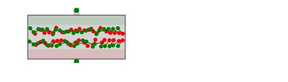
Shown above is the dielectric slab in the capacitor gap. The rotation angle of dipoles, which are shown as dumbbells with a red end and a green end, is animated. When the imposed electric field is large, they are aligned anti-parallel to the electric field. This is the effect of a dielectric slab in a capacitor: Since the slab’s dipoles align opposite to the imposed electric field they cancel a large fraction of that field and therefore a larger charge on the red and green plates is required to achieve the came voltage across the capacitor. When the imposed electric field is small or zero, the orientation of the dipoles becomes random as can be seen from the animation.

Summary

The meaning of equation (1.7) is that, if we initially charge the capacitor to value Q, then the subsequent charge will follow the product of the cosine periodic behavior times the exponential decay coefficient.