Atomic Model of Airfoil Lift and Drag

Introduction

In PhysicsAnimations.org under the chapter "Gas Physics", I've already shown that all of the statistical laws of gas physics can be obtained from numerical atomic models if atom-atom collisions are taken into account. In the present animation, I am showing that the standard laws of Airfoil lift and drag can also be reasonably obtained from numerical atomic models. What is new is that I show that a standard assumption, that the gas can be assumed to be incompressible, is not justified even for free stream flow rates that are much lower than Mach 1. In fact, the argument that the lift is due to the differences in density (compression) between the bottom of the airfoil and the top, seems to be justified for a particle approach like the present one.

Figures

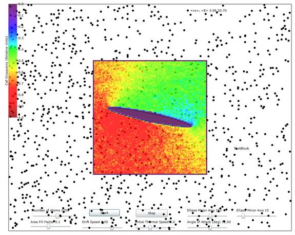
Figure 1: Showing the cell occupancy (average density) when the drift speed is about 60% of the mean thermal speed and with a 12 degree angle of attack. The relative scale for the density is shown in the color stripe at the left.

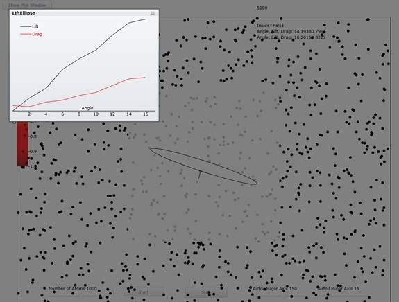
Figure 2: Showing the lift and drag Vs angle when the drift speed is 60% of the average thermal speed from 0 to 16 degree angle of attack. Note the characteristic linear relation for the lift and quadratic relation for the drag.

Physics and Math of Particle Approach

In other topics under the chapter "Gas Physics" I've documented the physics of particle-wall collisions and of particle-particle collisions. So here I will confine my remarks to atom collisions with the airfoil. For simplicity I've chosen a thin ellipse as my airfoil shape. Any thin section will result in approximately the same lift (albeit a bit more drag) as a "real" airfoil so a thin ellipse is a good compromise between realism and simplicity.

Since the atoms are flowing (drift speed) rather than the airfoil moving, the wing does not give up energy to the atoms and that means that their collisions with the wing conserve energy. To conserve energy, the two orthogonal components of the exiting atom's velocity must have the sum of their squares equal to the sum of the squares of the incident velocity components. For a smooth surface, the usual assumption is that the exiting velocity component tangential to the airfoil surface is the same as the incident tangential velocity component. That means that the exiting velocity normal to the airfoil has to be opposite to the incident velocity component. On a very fine spatial scale, no surface is smooth with respect to the de Broglie wavelength of the atoms (approximately 0.05 nanometers for air at room temperature). However, the assumption above will represent a reasonable average for the behavior of the atoms that hit the airfoil.

Computing the Normal Vector at the Impact Point

To compute the response of the atoms using the above assumptions, we need to be able to compute the normal vector of the ellipse at the point where the atom collides. Below, I will show how to compute this vector for any ellipse that is tilted at angle α with respect to the x axis.

Let the ellipse be centered at the origin of the (x,y) coordinate system and have semi-major axis a and semi-minor axis b. First we compute the angle of a prospective impact point with respect to this coordinate system.

$θ_{x y} = \tan 2^{- 1} (y, x)$

(1.1)

where the function tan2^-1 computes the angle on the range (-π,π).

Define the following values:

$\begin{array}{l} s_{y} = a \sin (θ_{x y} - α) \\ s_{x} = b \cos (θ_{x y} - α) \end{array}$

(1.2)

Now define some values that will let you compute the angles for the parametric description of the ellipse.

$θ_{p a r a} = \tan 2^{- 1} [s_{y}, s_{x}]$

(1.3)

At the same time, s_y and s_x are convenient for computing the distance from the center to the boundary of the ellipse at angle θ_xy.

$r (s_{x}, s_{y}) = \frac{a b}{s_{y}^{2} + s_{x}^{2}}$

(1.4)

In the un-tilted frame of reference, the normal vector is parallel to the following vector:

$N = a \cos (θ_{p a r a}) x + b \sin (θ_{p a r a}) y$

(1.5)

To become a useful unit vector N should be normalized as follows.

$n = \frac{a \cos (θ_{p a r a}) x + b \sin (θ_{p a r a}) y}{\sqrt{a^{2} \cos^{2} (θ_{p a r a}) + b^{2} \sin^{2} (θ_{p a r a})}}$

(1.6)

Now it is necessary to rotate n back to the angle of the ellipse in the coordinate system by applying the following rotation matrix:

$n_{x y} = (\begin{matrix} n_{x}' \\ n_{y}' \end{matrix}) = (\begin{matrix} \cos α & - \sin α \\ \sin α & \cos α \end{matrix}) (\begin{matrix} n_{x} \\ n_{y} \end{matrix})$

(1.7)

Using the Normal Vector to Compute the Lift and Drag Contributions at Each Impact

First we compute the dot product of the momentum vector with n_xy.

$p_{n} = n_{x y} • p$

(1.8)

Then we compute the change in the momentum vector

$δ p = 2 p_{n} n_{x y}$

(1.9)

The y component of this is the contribution to the lift, L

$δ L = δ p • y$

(1.10)

and the -x component of it is the contribution to the drag D:

$δ D = - δ p • x$

(1.11)

Comparison of Animation Results with Standard Equations

For 2 dimensional space, the standard equations for lift and drag of a thin symmetrical airfoil at low angle of attack are (see http://www.grc.nasa.gov/WWW/K-12/airplane/incline.html)

$\begin{array}{l} L \approx \frac{ρ}{2} v_{d}^{2} (2 π α) (2 a) \\ D \approx \frac{ρ}{2} v_{d}^{2} (2 π α^{2}) (2 a) \end{array}$

(1.12)

where v_d is the drift speed of the air along the x direction and ρ is the air mass per unit area. The result of equation (1.12) for the simulation, at, say 10 degrees or 0.16 radians, with 2a=300, v_d=2.5, ρ=0.00125 is L=1.29. The animation result for the same conditions is L=1.65. Therefore, the lift results for the animation are reasonably in agreement with the standard thin airfoil expressions.

Conclusions

Although the animation results in lift and drag numbers that are comparable to real world values, it is clear that some real world experiments that obtain difference in the speed of air flow over the top and bottom of the airfoil disagree with those obtained in the animation. Thus there must be a more complex interaction at the boundary layer at the surface of the airfoil. Since there are many real world cases where air viscosity can be neglected, we are left only with the (sub)microscopic roughness of the airfoil to explain how the airfoil re-shapes the contours of constant air velocity on its top and bottom.