Random Walk Animation

Introduction

Random walk determines a lot of processes in physics. For example, heat flow from a localized hot region into surrounding cooler regions can be described by random walk. For this animation we will show how random walk builds up a gaussian distribution probability of locations of a one dimensional position vector.

Math

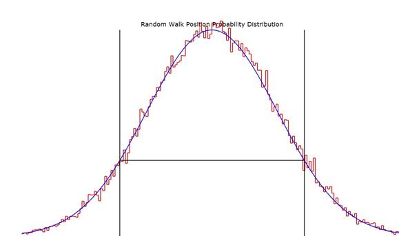
Random walk is a process where an entity has equal probabilities of stepping in either the positive or negative direction. For concreteness, let's call the entity a particle. This might at first seem to dictate that, after many steps, the particle would not have made any progress. That does happen to be the most likely result but there are many other cases where the particle actually displaces from its starting location. What we will show is that the ensemble (frequency distribution) after many trials of particle positions is a gaussian and the width of that gaussian is square root of twice the number of steps, n_s, each particle takes times the particle step size, δx.

$P (x, n_{s}) = \frac{1}{\sqrt{2 π n_{s} δ x_{}^{2}}} \exp (- \frac{x^{2}}{2 n_{s} δ x_{}^{2}})$

(1.1)

If the time rate of steps in ${\dot{n}}_{s}$ dn/dt then we can re-express equation (1.1) as a function of time, t:

$P (x, t) = \frac{1}{\sqrt{2 π {\dot{n}}_{s} t δ x_{}^{2}}} \exp (- \frac{x^{2}}{2 {\dot{n}}_{s} t δ x_{}^{2}})$

(1.2)

Figures

Plot of both the randomly computed distribution (stepped trace) and the proposed gaussian fit (smooth curve) to that distribution. The vertical lines show the position x= $δ x \sqrt{2 n_{s}}$ while the horizontal line shows the 1/e position on the smooth curve.

Relation to Heat Flow

In the case of heat flow in solids, the particle is the phonon and it random walks from higher temperature regions to lower temperature regions. The result above corresponds to the case where there is, initially, a nonzero temperature, T₀, at x=0 and zero temperature at all other locations. In that case the solution to Poisson's equation for the time and spatial function describing the temperature is

$T (x, t) = \frac{T_{0}}{\sqrt{4 π κ t}} \exp (- \frac{x^{2}}{4 κ t})$

(1.3)

$κ = \frac{K}{C_{V}}$

(1.4)

where κ is the diffusivity (conductivity, K, divided by the heat capacity per unit volume, C_V) and t is time. If we compare equation (1.3) with (1.2) we see that they are the same with the exception that, ιν εθυατιον 1.3, Τ0=1 ανδ 2κ = ${\dot{n}}_{s} δ x^{2}$ .