Thermal Conductivity and the Evolution of the Second Law of Thermodynamics

Introduction

This animation shows the exchange of energy of three adjacent gas domains at the two impermeable boundaries between them. The impermeable boundaries are needed in order to keep the atoms from the warmer region from simply diffusing into the cooler region. So, in effect, our three regions are solids that can exchange energy with the adjacent region but don't lose any of their atoms to that region.

In a previous animation we showed that the more energetic gas atoms, on average, give up during collisions, some of their energy to the less energetic gas atoms. That is exactly what happens at the boundary between two gas domains where the respective gases have different energies (or, equivalently, different temperatures). This results in heat energy flow from the higher temperature domain to the lower temperature domain. It is shown in the Appendix that the flow of energy from more energetic particles to less energetic particles occurs even for particles of different mass. This is a statement of the second law of thermodynamics for microscopic bodies. When I apply the same principles to whole regions of higher energy (temperature) then this shows the evolution of the second law of thermodynamics for macroscopic bodies as advertised in the title.

In this document, I will first give the standard thermal conductivity treatment for the three slabs of which this system is comprised. Then I will document on a more microscopic basis the dynamics how the time-dependent temperature distributions are achieved. In the Appendix I show the mathematics of the velocity changes when two particles of different mass and arbitrary velocities collide.

Figures

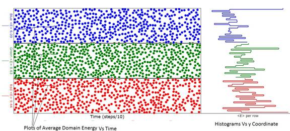
Figure 1: Diagram of the animation considerably before energy (temperature) evolution was complete. Note that the average energy (temperature) of the red domain exceeds that of the green domain and the green domain average energy exceeds that of the blue as can be seen from the ordinate labels at the left of the domains. In this animation the green domain had 600 atoms while the red and blue domains had 500 atoms. If you look closely, you will see that the boundaries between the domains are "puckered" when one of the atoms of a domain transgresses into the other domain. Sometimes when this happens, the transgressing atom collides with an atom in the other domain exchanging energy with it. That is the essence of how heat is exchanged between domains.

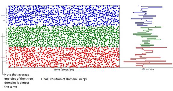
Figure 2: Diagram of the animation when energy (temperature) evolution was reasonably complete. Note that the average energy (temperature) of the three domains is almost the same as can be seen from the ordinate labels at the left of the domains. The differences are due to the finite number of atoms.

Animation Setup

For simplicity I have chosen to have just three domains arranged as layers. The top and bottom layer can be considered to represent solids. In solids, quantum entities known as phonons carry heat via vibrational modes. Phonons behave much the same as the kinetic energies of atoms so their equilibration and exchange of energies is reasonably represented by the kinetic energy of atoms. For even more simplicity I have chosen the number of atoms in the top and bottom layers to be the same so, when their average energies (temperatures) are equal, the thermal conductivity of these layers will be the same. To make the problem more interesting, the learner may select (within limits) the number of atoms in the middle layer and this will make the thermal conductivity (and heat capacity) of that layer different from the other two.

Macroscopic Temperature Calculations

To compute the temperature distributions Vs time we need to have access to two parameters:

1. The thermal conductivity, K (Watts m^-1 Kelvin^-1)

2. The heat capacity, C (Joules m^-3 Kelvin^-1)

The ratio of K to C is called the diffusivity, D=K/C (m²/sec).

The temperature, T, Vs time, t, can be found from the differential equation:

(1)

where the first inverted delta on the left is the divergence and the second is the gradient.

Initial Conditions Matching with Complementary Solution

We need a solution to specify the transients that occur starting at t=0. For that we use a technique called "separation of variables" which I will explain next. We have the three equations:

(2)

We make the assumption that each of the Ts can be written:

Then equation 2 can be rewritten:

(3a,b)

where L is called the eigenvalue.

The solution for equation 3b

(4)

Describing the Initial Conditions

We have three layers of thickness L₁, L₂, and L₃ and temperatures T₁, T₂, and T₃.

The initial temperature, T_i, Vs y can be written piecewise (denoted by subscript p) as:

(5)

Similarly the diffusion coefficient D can be expressed piecewise as:

(6)

In order to solve the differential equation we need to express T_p and D_p as periodic on the interval P=L₁+L₂+L₃ where P is the period of what will be the Fourier series describing T(y) and D(y). The series expressing T_i is:

where

It is quite easy to perform the integral for g_n:

Note that the average value of T is equal to g₀

Equations 5 and 6 have the problem that their first and second derivatives with respect to y are infinite at the interfaces between the layers. That can be rectified by using a "soft" step function at the interfaces. This step function is implemented by using 1/2 period of a sine wave.

where w is 1/2 of the width of the step, y₀ is the center of the step, T_avg=(T_a+T_b)/2, and T_diff=(T_b-T_a)/2 where T_a is the temperature at the start of the step and T_b is the temperature at the end of the step. Similar expressions can apply for steps in D. The step function must be applied at the transition between T₁ and T₂, T₂ and T₃ and for the transition from T₃ back to T₁. This results in a more complicated function T_p(y) and it is necessary to do the integrations for g_n numerically.

Case 1:D is the same in all layers:

The second derivative of T_i with respect to y is:

If D is the same in the 3 layers then we can immediately write that

so that

The results for T Vs t at various y values are shown in Figure 3 below:

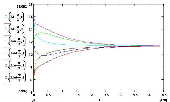
Figure 3: Temperature Vs time at several locations near the temperature transition boundaries computed using alternative software. Note the very high rates of change of temperatures near t=0. Note that the second and third curves are not even monotonic in their progress toward their final value. This is due to the very large gradient at the zone boundaries. This result is in good qualitative agreement with a similar finite element analysis.

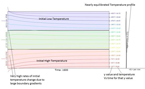
Figure 4. Temperature Vs Time obtained when the "Macroscopic" button is pressed. Note the very high rates of initial temperature change due to large initial boundary gradients. The 15 traces are displaced so that their final )equilibrated temperature ordinates lie at the y value for which that trace stands. In the green region, note that the slope of the temperature Vs time actually changes sign as it progresses toward equilibrium. That is due to the fact that it is initially adjacent to a much cooler or hotter region.

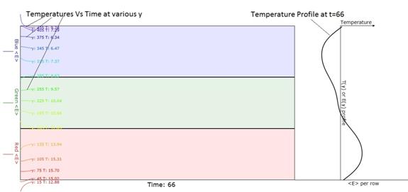
Figure 5. Earlier version of Figure 4. This shows a better description of the temperature profile at the right.

Case 2: D is different in all layers

In exactly the same manner we can write a Fourier series to express D_p:

It is important to know that our simple tri-level functions are adequately expressed for absolute values of n that are less than 50.

The first derivative of T_i (y) including the D term in equation 2 is:

The final y derivative in equation 2 results in:

This equation shows that a complicated function of y (the f terms) has taken the place of the previous constant eigenvalue. We could use perturbation theory to determine the effects of the variation of D on the original eigenfunctions. But that will be beyond the scope of this document.

Energy Distribution of a Gas

1. Standard Thermal Physics Treatment

The Boltzmann probability law for particle height, in a gravity (or acceleration field), g, is:

(1)

where N₀ is a normalization constant, m is the mass of the atom, k is Boltzmann's constant, v is the speed of the atom, and T is absolute temperature. It is easy to show that the average value of E, <E>, or mv²/2 is equal to kT using the integral:

Appendix

Particle-Particle Collisions of Different Mass and Velocity

The following will prove that, via particle-particle collisions, energy always flows from more energetic particles to less energetic particles. In order to have heat flow (thermal conductivity) from hotter (more energetic) regions to colder (less energetic) regions it is necessary that the previous statement be true.

Here we will consider spherical particles which have the different masses, m₁ and m₂, and diameters, D₁ and D₂. The centers of the spheres will be labeled (x₁,y₁,z₁) and (x₂,y₂,z₂). Upon collision, the momentum transferred between the spheres will always be along the unit vector:

(2)

where

is the distance between centers. Since the animation is illustrated in only 2 dimensions, the collision analysis will assume a containing box that is large in the x and y dimensions but very thin in the z dimension.

The expression for the final momenta in terms of the initial momenta is:

(3)

where the apostrophe on the left side of the equations indicates the final velocities. We know that the energies are conserved so

(4)

The directions of the change in momenta are along the vector of centers, u, and the values of the changes of momenta must be equal and opposite.

(5)

where M has units of mass and is still to be determined. Then

(6)

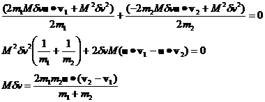
Now we can use equation 6 in equation 4 to solve for the value of Mdv.

(7)

where the large dot stands for the dot product and equation 7 simplifies to:

(8)

We can now make the identification:

(9)

where M is known as the "reduced mass".

Equations 6 and 8 are a complete solution for the final momenta. The final velocities are computed by dividing both sides of equations 6 by their respective masses:

(10)

Suppose m₂>m₁. Then we see that the magnitude of the speed added to molecule 1 will be larger than the magnitude of the speed removed from molecule 2. We can easily see from equation 7 that, even though the averages of the dot products are zero, that the collision results in an increased kinetic energy for molecule 1 and a decreased kinetic energy for molecule 2 because of the mass term in the denominators. Rewriting equation 4 we have:

(11)

If the initial speeds are the same then the only difference between E₁ and E₂ is due to the M² term in the kinetic energies.

(same speeds)

If the speeds are different, say v₂>v₁, but the masses are the same, then the difference in kinetic energies is due to the Mm term in the kinetic energies:

The above equation can be re-written:

where

is the cosine of the angle between v_i and u. The average value over all possible angles between v_i and u of the cosine squared terms is 1/2 so we can write

(same masses)

Therefore, averaged over all possible angles between u and v, the change of kinetic energy for particle 1 will be positive since v₂>v₁.

This degradation of the energy of the larger mass or higher speed atoms and/or speed leads to what is called the zeroth law of thermodynamics-all energy distributions tend to be become equalized. An example of this would be two gases of different molecular masses as well as different temperatures injected into an insulated box. The gas temperatures (or average energies) will equalize leaving the average speed of the gas with more massive molecules less than that of the gas with less massive molecules but the energies will tend to become equal due to the energy Vs velocity law we just proved.

Again rewriting equation 4 we have:

(12)

Let's compute the E₁ and E₂ for the general case where both m and v are different.

(13)

Inserting the expression for Mdv we have:

(14)

Rewriting equation 14 where I've explicitly given the expression for dv we have:

where v₁ and v₂ with the carats over them are unit vectors in the direction of v₁ and v₂, respectively. Their dot products with u are just the cosine of the angle between them and u and will be denoted c₁ and c₂.

(15)

It's clear that, over many collisions, the c₁c₂ terms average to zero.

Then the following expression for the average change of the energies per collision will be valid

(16)

Note that

(17)

(18)

The average value of c₁² and c₂² over very many collisions is 1/2 so we can rewrite this as

(19)

and then recognizing that the quantities in brackets are the original energies we have

(20)

From this equation we can say:

1. If E₂>E₁ the energy of particle 1 increases by a factor proportional to the difference.

2. If E₁>E₂ the energy of particle 2 increases by a factor proportional to the difference.

We may also subtract the above equations to write the differential equation:

(21)

where dn is the increment in the number of collisions and the equation has the solution:

(22)

where (E₁ - E₂)₀ is the initial value of the energy difference. The above equation shows that the energy difference between atoms 1 and 2 will degrade to zero as the number of collisions, n, increase. This result is for only one pair of atoms that interact by atom-atom collisions in a box. But this results also extends to the energy distribution of many atoms of possibly different masses colliding inside a box.

Removing Particle Overlap

Since the animation is digital we can expect that most often the collision condition will be realized when the distance between the centers of the two spheres,r₁₂, is less than D=(D₁+D₂)/2. To handle this I will increase the distance between the centers by the difference

by shifting each sphere in opposite directions by dr/2 along u. Thus we will move the centers of each particle by the vectors:

(23)