Use of Uniform Random Number Generator to Access a Weighted Probability Distribution

Introduction

            The impetus for this document is an electron diffraction animation.  I wanted to show the buildup of the wave-directed electrons in the far field of a slitted screen upon which electrons are incident one-by-one.  After many electrons have passed, the envelope of the histogram of number of electrons Vs far-field angle will be a product of two sinc functions.  This is the weighted probability distribution of the title.

Method

            The method that I came up with is to compress the algebraic distribution.  Each of the blocks in the new index distribution will have a width proportional to the value of the probability that that block represents. This way, when we choose uniform random variables on the entire numerical domain of the blocks, we will be choosing fewer values where the original probability was low.  See the start of a numerical example below where the top row of numbers represents index of the abscissa of the function and the second row represents the compressed indices from which to choose random numbers.

Example with a Gaussian Distribution

            Let the original distribution be written as:

$$\frac{dP(x)}{dx}=\frac{1}{\sqrt{\pi }\sigma }\exp \left(-{\left(\frac{x-x_0}{\sigma }\right)}^2\right)$$

(1)

where σ is the width at 1/e of the distribution and dP/dx is the probability that x will be in the interval dx.

 

We will remap the numbers describing the distribution such that the range of numbers corresponding to P(x) is proportional to the value of P(x).  i.e.

dN(x)/dx=N_T dP(x)/dx and make N_T>>1_.

i.e.

$$k_i=N_T{\displaystyle \sum _{n=0}^i\frac{dP}{d{x}_n}}$$

where x_n varies in units of (x_max-x_min)/N_T. Having computed k_i, and saved it to an array then we use the computer’s uniformly distributed random number generator to select a number, g, from the range 0 to k_max.  Then we use the following algorithm to compute the i value to which g corresponds:

int i=0;

                     do

                     {

                           i++;

                     }

                     while(k[i]<g);

                     return i;   

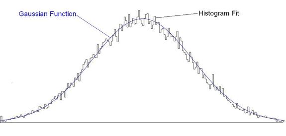
The final result appears as shown in Figure 1:

Figure 1: Both the original Gaussian probability distribution and the weighted profile (really a frequency distribution) generated by the compression technique described above.