Spreadsheet 0: Frequency of a Charge Displaced
3 Angstroms
3 Angstroms
Hover over the menu bar to pick a physics animation.
`(d^3P)/(dAdOmegadf)=(2 f^2)/c^2 (hf)/(e^((hf)/(k_BT_K))-1) (1)`
where `(d^3P)/(dAdOmegadf)` is the power per unit area emitted into a 1 Hz band width and into unit solid angle. Here f is the frequency, c is the speed of light in vacuuum, `T_K` is the absolute temperature, `k_B` is Boltzmann's constant and h is Planck's constant. At first glance it looks as if `(d^3P)/(dAdOmegadf)` goes to infinity for `(hf)/( k_BT_K)->0` and finite temperature, but if we expand the exponential in the denominator for `(hf)/( k_BT_K) "<<"1` we see that `(d^3P)/(dAdOmegadf)` becomes`(d^3P)/(dAdOmegadf)((hf)/( k_BT_K) "<<"1)=(2 f^2)/c^2 k_BT_K (2)`
It is important to define what we mean by a black body: It is a surface that absorbs all radiant energy falling on it. The term 'black' arises because incident visible light will be absorbed rather than reflected, and therefore the surface will appear black. However, for an isolated system, the energy will generally be re-emitted at longer wavelengths. The temperature `T_K` can be achieved by radiation at any wavelength. Or it can be achieved by heating with a resistive heater and the resulting emission spectrum will not change. A black body may be either a flat black surface or a cavity with a very small hole in it to permit observation of the radiation spectrum. For the present simulation we will assume a black surface that contains many quantum harmonic oscillators. Max Planck's early papers on his radiation law assumed many different non-interacting oscillators whose frequencies spanned the black body radiation spectrum. Later he had to accept that any oscillators had to interact with oscillators of different frequency. Otherwise, if the black body was heated by applying radiation at only one frequency, how would the oscillators at all the necessary frequencies of the black body frequency distribution re-radiate? Actually we could assume damped harmonic oscillators since we know that they will eventually lose their energy to heat. Take the example of the quartz crystal oscillator in your wrist watch 1. Its Q factor is about 25,000 which means that it oscillates about `25000/(2pi)` cycles before its kinetic energy is reduced to 1/2 of its original value. This energy will heat its surroundings just as radiant energy heats a surface around where it is absorbed. For damped (interacting) quantum oscillators the math gets very cumbersome 2 so here we will just animate classic harmonic oscillators.
To do that, we first need to know the classic power output of a single charge (or dipole) vibrating at frequency f. The vibrating charge will be called a dipole and its carrier can have the mass of just an electron or it can have the effective mass of one atom of a polar molecule. An example of a polar molecule is carbon monoxide (CO) which has a dipole moment of `0.122 D` (Debye where a Debye is 0.0208 electron nm) for which CO dipole moment works out to 0.0025 electron nm. Then we need to choose a surface number distribution of these charges that can result in the power per unit frequency bandwidth given in equation 1. The power per unit solid angle averaged over `4pi` steradians at frequency f and with a dipole moment `p_0` is the following expression:
`(dP)/(dOmega)=pi^2 p_0^2 /(3 epsilon_0) f^4/c^3(3)`
where `p_0` is:` p_0=e d`
where `e` is an electron charge and `d` is the amplitude of its motion.`(dP)/(dOmega)=pi^2 f p_0^2 /(3 epsilon_0 lambda^3)(3a)`
We know that a term like`(Qq)/(4 pi epsilon_0 r)`
is the potential energy of charge q at distance r from charge Q. Then equation 3a has the same dimension except the potential energy is multiplied by frequency f and becomes energy per unit time and is power which is what wanted to prove.`(d^2P)/(d Omega df)=4/(3epsilon_0) pi^2 p_0^2 (f^3)/c^3 (4)`
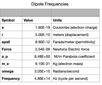
Next we should consider what the dipole frequency might be. The typical dipole electron bound to a much more massive nucleus of the same but oppositely signed effective charge has an amplitude of order `d=3cdot10^-10` meters which results in a force of (see Spreadsheet 0)
`F= e^2/(4 pi epsilon_0 d^2)=2.5 cdot 10^-9 " Newtons"`
For this animation, since I want to adjust frequency easily, I will model the electron potential, V, as that of a harmonic oscillator. The harmonic oscillator also has the advantage that the temperature dependence of its energy distribution is the same as that in the Planck black body emission equation. In fact the energy distribution of an assembly, N, of harmonic oscillators is`U(f,T)=Nhf(1/2+1/(exp((hf)/(k_BT_K))-1))`
Our definition of the harmonic oscillator potential is:`V=a_p/2 d^2`
so the force is:
`F=-a_p d`
` a_p=(2.5 cdot 10^-9)/(3 cdot 10^-10)=8.5` Newtons per meter.
Then the radian frequency is
`omega=sqrt(a_p/m_e)=sqrt((8.5)/(9.1 cdot 10^-31))=3 cdot 10^15`
and the cycles per second are:
`f=omega/(2 pi)=4.9 cdot 10^14 Hz`
We have seen that the factor `k_BT_K` always corresponds to the average kinetic energy, `KE` of the particles of the system. The average kinetic energy is a sum over all `KE_i` of the system:
`KE_("average")=1/n sum_1^n(KE)_i`
In the present simulation, the only significant kinetic energy is that of the vibrating electrons or polar atom. Therefore one requirement of the numerical matching of the Planck black body equation (1) is that the denominator of the equation read:
`k_BT=1/n sum_(i=1)^(i=n)(KE)_i`
`e^((hf)/(k_BT))-1=e^((hf)/(1/n sum_1^n(KE)_i))-1`
But what is the form of `KE_i`? It is related to the oscillator frequency and displacement in a simple way. The maximum value of KE is the same as the peak value of the potential energy.`KE_(max)=1/2 a d^2=1/2 m_e omega^2 d^2=2 pi^2 m_ef^2 d^2`
and, of course, the time average kinetic energy is 1/2 of `KE_(max)`. Then the denominator in the both the Planck equation and dipole energy power equation becomes:`e^((hf)/(k_BT))-1=e^((hf)/ (pi^2 m_e/n sum_1^n(f_id_i)^2))-1`
To match the frequency distribution we have to choose a dipole areal density and power distribution `n(f_i)P_i` that agrees with equation 1. So we have the following equation:
` (dn)/(dA)(d2P)/(dfdOmega)=(4pi^2)/(3epsilon_0) p_0^2 (f^3)/c^3=`
`(2 f^2)/c^2 (hf)/(e^((hf)/(k_BT))-1) (6)`
`(dE)/(dhf)=(1/2+1/(exp((hf)/(k_BT))-1))`
and we can ignore the `1/2` since that is the zero point energy and can't participate in emission. Then equation 6 becomes:
` (dn)/(dA)(d2P)/(dfdOmega)= (dn)/(dA) hf(1/(exp((hf)/(k_BT))-1))(4pi^2)/(3epsilon_0) (f^2)/c^3 p_0^2=`
`(2 f^2)/c^2 (hf)/(e^((hf)/(k_BT))-1) (6)`
` (dn)/(dA) (1/(exp((hf)/(k_BT))-1))(4pi^2)/(3epsilon_0) (ed)^2 f^3/c^3= (2 f^2)/c^2 (hf)/(e^((hf)/(k_BT))-1) (6a)`
We have some options of choice of parameters to cause this equation to be valid. We can choose the distributions of the dipole lengths `d` and we can choose dn/dA. The dipole lengths `d` change the kinetic energy distribution which is the same as changing the effective temperature. So we are left with computing `(dn)/(dA)` to satisfy equation 6a.` (dn)/(dA)= h(epsilon_0)/(4pi^2 (ed)^2 f/c) (7)`
`d^2=d_0^2lambda/(lambda_0)=d_0^2(f_0/f) (8)`
so we just need to choose fairly small total area and satisfy equation 8 at random sites.1. The center of mass of the dipole must not move during its oscillation cycle
2. The net charge of he dipole must be zero
The first requirement results in the oscillation displacement of the end masses being inversely proportional to their masses and opposite in direction with respect to their center of mass. The second requirement just means that the dipole molecule is not ionized. A third aspect is that the dipole orientation is random since there is no reason to assume the entire surface is a crystal. Assume that the orientation of a given dipole is `phi` and the static separation is `d_0` and the end masses are `m_1` and `m_2`. Then the static position of its charges with respect to its center of mass (CM) is
`x_1=m_2/(m_1+m_2)d_0 cos phi`
`y_1=m_2/(m_1+m_2)d_0 sin phi`
`x_2=-m_1/(m_1+m_2)d_0 cos phi`
`y_2=-m_1/(m_1+m_2)d_0 sin phi`
`x_1=m_2/(m_1+m_2)(d_0+a cos theta) cos phi`
`y_1=m_2/(m_1+m_2)(d_0+a sin theta) sin phi`
`x_2=-m_1/(m_1+m_2)(d_0+a cos theta)cos phi`
`y_2=-m_1/(m_1+m_2)(d_0+a sin theta) sin phi`
`bb p=-2e(m_2-m_1)/(m_2+m_1)a cos theta bb hat d_0`
where bold letters denote vectors and `bb hat d_0` is a unit vector in the direction of the vector `bb d_0`. Then, if `m_2 ">" m_1` and the charge on `m_2` is `+e` as one might expect, and `a cos theta>0`, the direction of the dipole moment is opposite that of `bb hat d_0`. A group of animated dipoles is shown on Canvas 1.Dipole photon emission occurs randomly and its energy Vs frequency spectrum follows the Planck spectrun in equation 1. Canvas 0 shows the accumulation of photon energies in bins that finally match the Planck spectrum Also shown are the colored fill and smooth plot there. In order to show random filling of the bins, a special mapping onto integers of the frequency spectrum curve was done using the function mapKs().
The same mapping was done to randomly specify the frequencies of the animated dipoles in Canvas 1. The amplitudes of vibration of the dipoles was according to equation 8. Canvas also 1 shows random emissions in the form of lightning bolts and their color corresponds to the wavelength associated with the frequency of oscillation of the dipoles.