Quantum Modes of Particle in a 1D Mexican Hat Potential
The goal of this program is to explore the boundary between classical physics and quantum physics. This boundary was first hypothesized by Niels Bohr in 1920 and is called the Bohr Correspondence Principle . To do this I will show the classical motion of the particle at the eigenmode energy as well as the usually periodic variation of the particle wave function in this eigenmode. The modes are the eigenvalues and eigenvectors of the second order Schrodinger equation (SE)
`-(ℏ^2)/(2m)(del^2Psi)/(delx^2)+V(x)Psi=EPsi`
, where ℏ is the reduced Planck constant, m is the mass and E is the energy of the particular mode whose wave function is the eigenvector. The reader might want to refer to Finding Eigenvectors from Eigenvalues.
For this program I have chosen to set the Planck constant (divided by 2*pi), ℏ, equal to
1 Joule second and the mass, m, equal to 1 kilogram.
Although the SE can also express the time dependence of the wave function,
only the steady state eigenmodes will be computed here.
The second derivative operator can be expressed in tridiagonal matrix form as
The entire matrix expression of the time independent SE is then 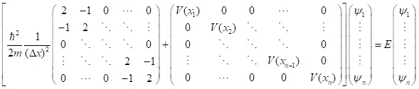 In order to solve this equation efficiently using the Jacobi Method,
I have derived Jacobi Method Modifications.
The potential V(x) here is a standard harmonic oscillator parabola with a guassian "bump" in the middle so it looks like an upside down Mexican hat.
This potential is believed to be the "symmetry breaking" feature that mediates the Higgs boson in the Standard Model of quantum field theory.
Of course the potential in quantum field theory is 3 dimensional but three dimensions are hard to depict so I have chosen 1 dimension, x, here.
As labeled, the black trace is the potential that the particle is in, the red trace is the force it feels at any given location,
the orange trace is the signed velocity of the particle,
and the green trace is the time spent per unit distance moved by the particle, 1/|Velocity|.
The latter would equal the value of the magnitude squared of the wave function for very large wave function quantum numbers.
The green trace value should be proportional to the envelope of the square of the quantum mechanical wave function, psi,
for the quantum mode which corresponds to the initial potential energy of the particle.
But in quantum field theory, the particle will sometimes "tunnel" through the center hill of the potential, so a simple relation to the classical value if 1/|vx| cannot be expected.
The eigenvalues of the particular setup are depicted as a purple trace with small purple circles at each eigenvalue.
By placing the mouse on one of these circles, and clicking the eigenvector (spatial mode) of that
eigenvalue will be drawn in a color corresponding to the index number of the eigenvalue.
If this circle is clicked again, the eigenvector corresponding to that eigenvalue will be removed from the list of drawn eigenvectors, reducing the clutter so that new eigenvectors can be viewed.
The eigenvalues can be computed quite efficiently using the Jacobi method which successively "zeros out" the off diagonal elements
by simple two dimensional rotations. These rotations change only two rows and two columns of the matrix so, instead of full matrix multiplications,
we only need to compute the changes to these two rows and two columns.
In order to solve this equation efficiently using the Jacobi Method,
I have derived Jacobi Method Modifications.
The potential V(x) here is a standard harmonic oscillator parabola with a guassian "bump" in the middle so it looks like an upside down Mexican hat.
This potential is believed to be the "symmetry breaking" feature that mediates the Higgs boson in the Standard Model of quantum field theory.
Of course the potential in quantum field theory is 3 dimensional but three dimensions are hard to depict so I have chosen 1 dimension, x, here.
As labeled, the black trace is the potential that the particle is in, the red trace is the force it feels at any given location,
the orange trace is the signed velocity of the particle,
and the green trace is the time spent per unit distance moved by the particle, 1/|Velocity|.
The latter would equal the value of the magnitude squared of the wave function for very large wave function quantum numbers.
The green trace value should be proportional to the envelope of the square of the quantum mechanical wave function, psi,
for the quantum mode which corresponds to the initial potential energy of the particle.
But in quantum field theory, the particle will sometimes "tunnel" through the center hill of the potential, so a simple relation to the classical value if 1/|vx| cannot be expected.
The eigenvalues of the particular setup are depicted as a purple trace with small purple circles at each eigenvalue.
By placing the mouse on one of these circles, and clicking the eigenvector (spatial mode) of that
eigenvalue will be drawn in a color corresponding to the index number of the eigenvalue.
If this circle is clicked again, the eigenvector corresponding to that eigenvalue will be removed from the list of drawn eigenvectors, reducing the clutter so that new eigenvectors can be viewed.
The eigenvalues can be computed quite efficiently using the Jacobi method which successively "zeros out" the off diagonal elements
by simple two dimensional rotations. These rotations change only two rows and two columns of the matrix so, instead of full matrix multiplications,
we only need to compute the changes to these two rows and two columns.
From the Schrodinger Equation solutions we obtain three important types of information about how a particle moves in the potential V(x).
1. The energies, Ei, which are the eigenvalues of the stationary state modes.
2. The square of the amplitudes of the eigenvectors, vi, which is the probability density for the position, x, of the particle.
3. The spatial frequencies, k(x) Vs position x of the eigenvectors to which the particle momentum is proportional.
All three of these quantities are computed and displayed in this program except k(x) is not computed for eigenvalue mode numbers less than about 12.
The learner should note that the probability density is usually lower where the spatial frequency k(x) is higher as shown in the following Figure:
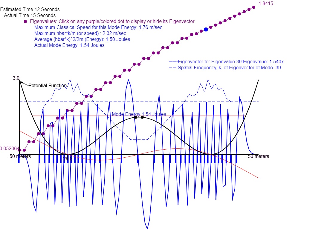
Figure 1: Eigenvector amplitudes and spatial frequencies k(x) of Eigenmode 39 where the total range of x was 100. Note that the k(x) is larger where psi(x) amplitude is smaller. Also note that the eigenvalues (energies) occur in pairs (doublets) of equal energy up to and including mode 35. This doublet behavior is called degeneracy. Degeneracy is where a mode has different spatial distribution but the same energy bevause of the symmetry of the potential energy. At mode 35 the mode energy is just below the center peak of the potential energy. All modes below that have equal probability of appearing mainly in the left or right potential well
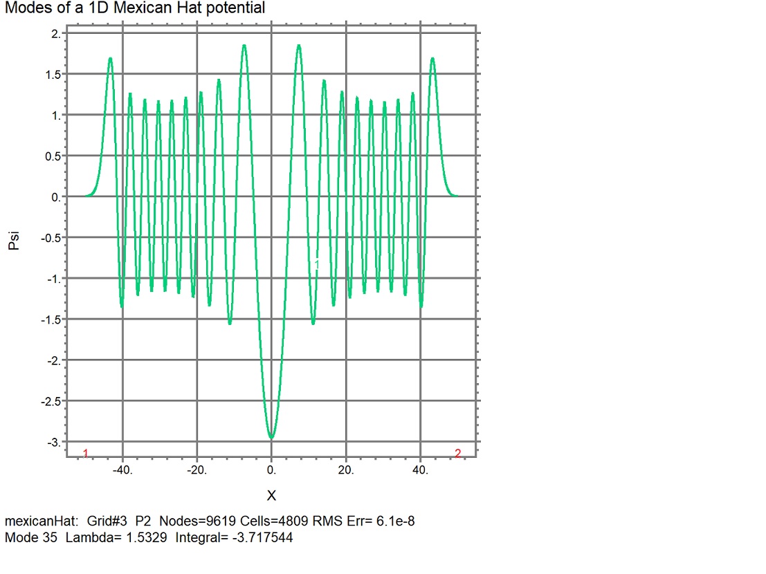
Figure 2: Eigenvector plot by finite element method (FEM) of Eigenmode 35 where all parameters except the mode number are the same as in Figure 1. Note that the periodic wavefore is much smoother than that of Figure 1. That is to be expected for the FEM since it uses many more spatial increments than the finite difference method (FDM). An important similarity between the two methods is that the transition from doublet energy modes to singlet modes (to non-degeneracy) occurs when the mode energy just exceeds the peak center potential.
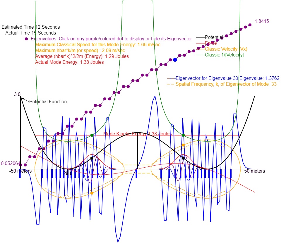
Figure 3: Similar to Figure 1 but with the classical velocity (orange), classical 1/|velocity| (green), and a gaussian wave packet (red) plotted. The quantum velocity is also plotted in orange with a dashed line. Note that the classic velocity and quantum velocity agree quite well. However, one would expect that the envelope of the magnitude squared of the eigenvector (blue) should agree reasonably with the classic value of 1/|velocity| At best one might say that there is qualitative agreement in that the x value of the maximum of the envelope coincides with the maximum of the 1/|Velocity| curve. One must conclude that the quantum effect is to greatly "soften" the infinite result for 1/|v| of the classical turn around at each end of the classic trajectory. Either that or one might argue that I have not chosen a large enough quantum number for the Copenhagen Interpretation (probability)to be valid. This softening is to be expected from the Heisenberg Uncertainty Principle since that principle would preclude determinining the exact point of turnaround. The gaussian wave packet moves in the x direction at the exact speed of the particles. If this wave packet were immersed in this potential there would be significant distortion near the ends of its trajectory. But this distortion is a subject of the time dependent Schrodinger equation and is reserved for a later animation.
Interpretation of Time Independent Schrodinger Equation Solution
Note that the solution is in the form of a standing wave. Since the wave is standing and has regularly spaced nodes, there can be only one way of interpreting it: The interference pattern of two oppositely traveing waves desceibed by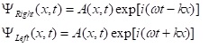
where A and k are constantly varying functions of x. Obviously this sum addes up to a cosine function in x. Classically this would correspond to oppositely moving particles of equivalent speed. That is what I show when the learner selects the "Start Particle Motion" button. We expect that that maximum classical speed should be equal to the maximum of the quantum product hbar*k where k is 2*pi/lambda and lambda is twice the space between zero crossings of the Schrodinger wave function, I provide a comparison of these two quantities and the difference is usually less than 10% of the average. Also, the average kinetic energy of the mode is its eigenvalue and we should expect that this eigenvalue should be equal to <|hbar*k|^2/(2*mass) where the <> symbols indicate average. The differennce between these two quantities is uusually less than 20% of the average of the quantities, This concludes my interpretation of the time independent wave function. Note that this interpretation is much more detailed than the Copenhagen Interpretration which usually only asserts that the magnitude squared of the wave function is the probability of that the particle will be in a given location. The learner has the option of downloading any of these graphics by right-clicking and selecting "Copy".