Spreadsheet 0: Gold Foil Target Spreadsheet
Hover over the menu bar to pick a physics animation.
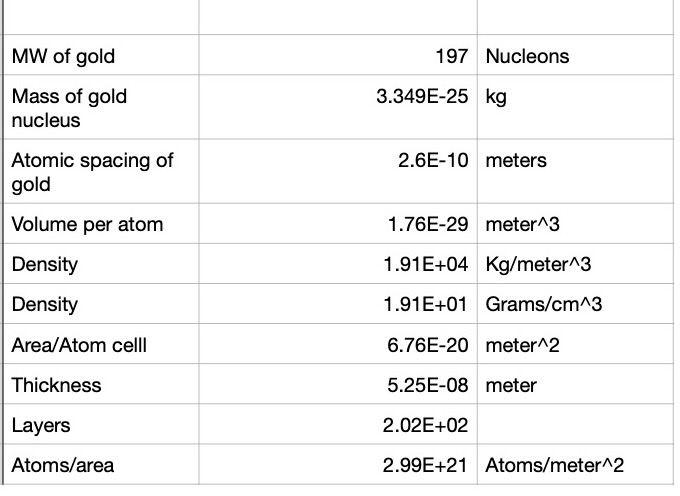
This animation is similar to the Rutherford scattering experiment. The Rutherford scattering experiment (RSE) is famous because it established that atoms of a solid have a very compact nucleus. In the case of the RSE, the solid was a very thin gold foil and the incident particles were doubly ionized helium atoms (nucleii) which are also called alpha (`alpha`) particles. The molecular weight of gold is 197 and that of helium is 4. Therefore, if almost all the mass of the gold atom is concentrated in its small nucleus, when the alpha particle hits the gold nucleus, only a small fraction of its energy will be transferred to the nucleus. If the alpha particle hits the gold nucleus dead center, then the alpha particle will bounce back 180 degrees from its original direction. It turned out that that is what happened. It led to Rutherford making the now famous comment:
"It was quite the most incredible event that has ever happened to me in my life. It was almost as incredible as if you fired a 15-inch shell at a piece of tissue paper and it came back and hit you."
This result would not have been the case if the nucleus were not extremely compact. It turns out that the nucleus mean radius is of the order `r_(n)=10^(-14) ` meters. Gold has a face centered cubic (FCC) crystal structure where the cube edge is `a_(gold)=4.07cdot10^(-10)` meters. So viewed from the side, as seen in Canvas 0, the spacing between each gold atom occupies an area of 1/2 the area of a square of edge length `a_(gold)` so each gold atom occupies an area `A_(gold)=(16.56/2)cdot10^(-20) meters^2` (see Spreadsheet 0) . This means that it will be extremely unlikely that a small alpha particle would have a hard collision with a helium nucleus. In fact, the probability, P, is about
`P=(pi r_n^2)/A_(gold)=3.5 cdot 10^(-9)`
and yet a significant fraction of the alpha particles were deflected at other than small angles. Part of the reason for that is that the alpha particle did not have to actually contact the nucleus of gold since both have fairly large positive charge. The charge of gold is `Z_(gold)=79` while that of the alpha particles is `Z_(alpha)=2` where the Z values represent the number of oppositely signed electron charges, `e`, where `e=1.6cdot10^(-19)` coulombs.
With that introduction, we are now ready to work out the details of this animation. The illustration in Canvas 0 shows only a single layer of gold nucleii. An actual gold foil will have at least `n_L=200` layers so the probability of a direct hit is increased by `n_L` or to `P=0.7 cdot 10^(-6)` if `n_L=200`.
`bb v_f=bb v_i-2 hat bb"u" ( bb v_i cdot hat bb"u") `
where `bb v_i` is the incident velocity and `hat bb"u"` is a unit vector pointing from the target particle to the beam particle. Note that this equation conserves energy
`(bb v_f cdot bb v_f) =(bb v_i cdot bb v_i)`
` -4 (hat bb"u" cdot bb v_i) ( bb v_i cdot hat bb"u")`
`+4 (bb v_i cdot hat bb"u" ) (bb v_i cdot hat bb"u") =(bb v_i cdot bb v_i)`
`x_p=x_p+v_xdt`
`y_p=y_p+v_ydt`
`s_t=2.5/(opacity)*(r_t+r_b)`;
where the 2.5 factor is just a parameter that seems to make the ratio of forward scatter to backscatter agree with the numerical results.`m_1 bb"v"_{1f}+m_2 bb"v"_{2f}=m_1 bb"v"_{1i}+m_2 bb"v"_{2i} (1)`
where the subscript f stands for final value and the subscript i stands for initial value and the arrowed bold letter ` bb"v"` stands for the velocity vector. The conservation of kinetic energy equation is as follows:`m_1 bb"v"_{1f} cdot bb"v"_{1f} +m_2 bb"v"_{2f} cdot bb"v"_{2f}`
`=m_1 bb"v"_{1i} cdot bb"v"_{1i} +m_2 bb"v"_{2i} cdot bb"v"_{2i} (2)`
where the `cdot` between the velocity vectors stands for the inner or dot product of the two vectors. When we combine equations 1 and 2 we get equations that relate the components of the velocity vectors.The most important concept in these calculations is that of the unit vector ` hat bb"u"` between the centers of the two particles that are colliding
` hat bb"u"=[(x_2-x_1)hat bb"x"+(y_2-y_1)hat bb"y"+(z_2-z_1)hat bb"z"]/r_{12}`
where the x, y, and z that have hats are unit vectors along their respective axes and`r_{12}=sqrt[(x_2-x_1)^2+(y_2-y_1)^2+(z_2-z_1)^2]`
Note that the unit vector points from sphere 1 to sphere 2 so, if `x_2` is greater than `x_1`, the unit vector's x component is positive.`m_1 delta bb"v"_1=M delta v hat bb"u"=-m_2 delta bb"v"_2 (3)`
where `M` has units of mass and `M` and the scalar speed increment `delta v` are still to be determined. Now we may re-write equation 2 using equation 3 and obtain:`((m_1 bb"v"_1+M delta v hat bb"u") cdot (m_1 bb"v"_1+M delta v hat bb"u"))/(m_1)+ ((m_2 bb"v"_1-M delta vhat bb"u") cdot (m_2 bb"v"_2-M delta vhat bb"u"))/(m_2) =m_1 bb"v"_{1} cdot bb"v"_{1} +m_2 bb"v"_{2} cdot bb"v"_{2}(3)`
After cancellations of the terms on its right side, equation 4 simplifies to:`M delta v=(2m_1m_2)/(m_1+m_2)( bb"v"_1- bb"v"_2) cdot hat bb"u"`
We can now make the identifications:`M=(2m_1m_2)/(m_1+m_2)`
and`delta v=( bb"v"_1- bb"v"_2) cdot hat bb"u"`
where M is known as the "reduced mass" Finally using equation 3 again we can write the expressions for the final velocity vectors:
` bb"v"_{1f}= bb"v"_{1i}+M/m_1 [( bb"v"_1- bb"v"_2) cdot hat bb"u"] hat bb"u" (5)`
` bb"v"_{2f}= bb"v"_{2i}-M/m_2 [( bb"v"_1- bb"v"_2) cdot hat bb"u"] hat bb"u"`
`r=r_1+r_2`
The next task for us is to relate these final speeds and energy changes to the collision parameter, `b`. First we can write the following equation for the unit vector `u` between the two spheres:`bb u=1/r[-(sqrt(r^2-b^2))bb (hat x)+b bb hat(y)]`
Thus`u_x=-sqrt(1-(b^2/(r^2))), u_y=b/r`
Without loss of generality, let's just have `bb v_1=v_1 bb (hat x)` and `bb v_2=0` and then use equation 5 to compute the final velocity.` bb"v"_{1f}= bb"v"_{1i}+M/m_1 [( bb"v"_1) cdot hat bb"u"] hat bb"u" `
Taking the dot product of `bb v_1` with `hat bb u` we obtain:
` bb"v"_{1f}= bb v_{1i}+M/m_1 [( v_1)/r[-(sqrt(r^2-b^2))]] hat bb"u" `
` bb"v"_{2f}= -M/m_2 [( v_1)/r[-(sqrt(r^2-b^2))]] hat bb"u" `
`v_(1fx)=v_(1i)(1-2[1-(b/r)^2])), v_(1fy)=-v_(1i)(2sqrt[1-(b/r)^2])b/r)`
Then the expression for the tangent of the angle of `bb v_1` is:`tan(phi_(sc))=-{2(b/r)sqrt[1-(b/r)^2]}/{1-2[1-(b/r)^2]}`
The scatter direction of particle 2 is along the `bb u` vector and the scatter direction of particle 1 is along the unit vector:` bb u_(1f)= {bb v_{1i}+M/m_1 [( v_1)/(r)[-(sqrt(r^2-b^2))]] hat bb u}/ (sqrt((bb (v_(1f)) cdot bb (v_(1f))))) (6)`
`(d Omega)/(d theta)=2 pi theta`
and then we can use an expression for `theta` to compute `(d theta)/(db)` and obtain:`(d Omega)/(d b)=2 pi theta (d theta)/(db)`
Now we need the expression for `(d theta)/(db)``(d theta)/(db)=(d)/(db)[tan^-1 (v_(1y)/v_(1x))]`
The derivative of `tan^-1(x)` is `1/(1+x^2) so we need the derivative:`(d theta)/(db)=(d)/(db)[1/(1+(v_(1y)/v_(1x))^2)]`
Following through with the derivatives of v with respect to b we have:`(d v_(1y))/(db)=-v_(1ix) [sqrt(r^2-b^2)/(r^2)-b^2 /(r^2 sqrt(r^2-b^2))]`
We may now use equation 5 to compute the direction of `bb v_(1f)` on the assumption that `m_2 gt gt m_1` which means that `M/(m_1)=2`:
`v_(1fx)=v_(1ix)-2v_(1ix)(r^2-b^2)/(r^2)`
`v_(1fy)=-2v_(1ix)b sqrt(r^2-b^2)/(r^2)`
`theta_(xi)=tan^-1(v_(1fy)/v_(1fx)))`
`theta_(iota)=tan^-1(b/sqrt(r^2-b^2))`
so that, when `m_2` is very large, the angle of exit with respect the `bb u` is just twice the angle of incidence with respect to `bb u`. From the angle result the number of particles that will scatter into a given solid forward or backward solid angle increment `delta Omega` can be computed similarly to the very important Rutherford scattering experiment where charged alpha particles scattered from heavy nucleii in gold foil. First note that from the definition of a solid angle:`(d Omega)/(d theta)=2 pi theta`
and then we can use our expression for `theta_xi` to compute `(d theta)/(db)` and obtain:`(d Omega)/(d b)=2 pi theta (d theta_xi)/(db)`
Now we need the expression for `(d theta_xi)/(db)``(d theta_xi)/(db)= 2(d theta_iota)/(db)=2/(sqrt(r^2-b^2)`
so that`(d Omega)/(d b)=(4 pi tan^-1(b/sqrt(r^2-b^2)))/(sqrt(r^2-b^2)`
`(d Omega)/(d b)=(4 pi theta_iota)/(sqrt(r^2-b^2)`
As always, the learner is encouraged to press F12 (Windows) and select "Sources" to examine the HTML and javascript code that was used to create this page.